Cumulative Cost and Budget Spreadsheet Tool
As both a Project Management practitioner and a College Professor and University Instructor, I have found that there are very few simple-to-use templates for creating a time-based project schedule and budget. This package has a series of 4 Excel spreadsheets (but any standard spreadsheet program should also work) that allow a student or practitioner to build a time-based budget that shows unit activity (scope) planned period (time), and cumulative cost all on one page. It has been created to demonstrate a fictitious but realistic budget for the purchase, installation, and testing of a mid-size local area network of about 200 desktop and laptop computers and 5 servers. The project is expected to take 15 weeks from start to finish with a total budget of $402,200.
4 spreadsheets in total allow readers to copy and build their budget.
Sheet 1,2,3 shows the building blocks of creating a time phase schedule for buying and installing laptops, desktops, and servers. Unit activity and planned unit prices drive the planned equipment budget. Similarly, there are a few human resources planned with daily labour rates driving the total labour cost plan. The summary cost lines from the equipment and labour detail sections are then summed to yield the total planned cost for each week and cumulatively.
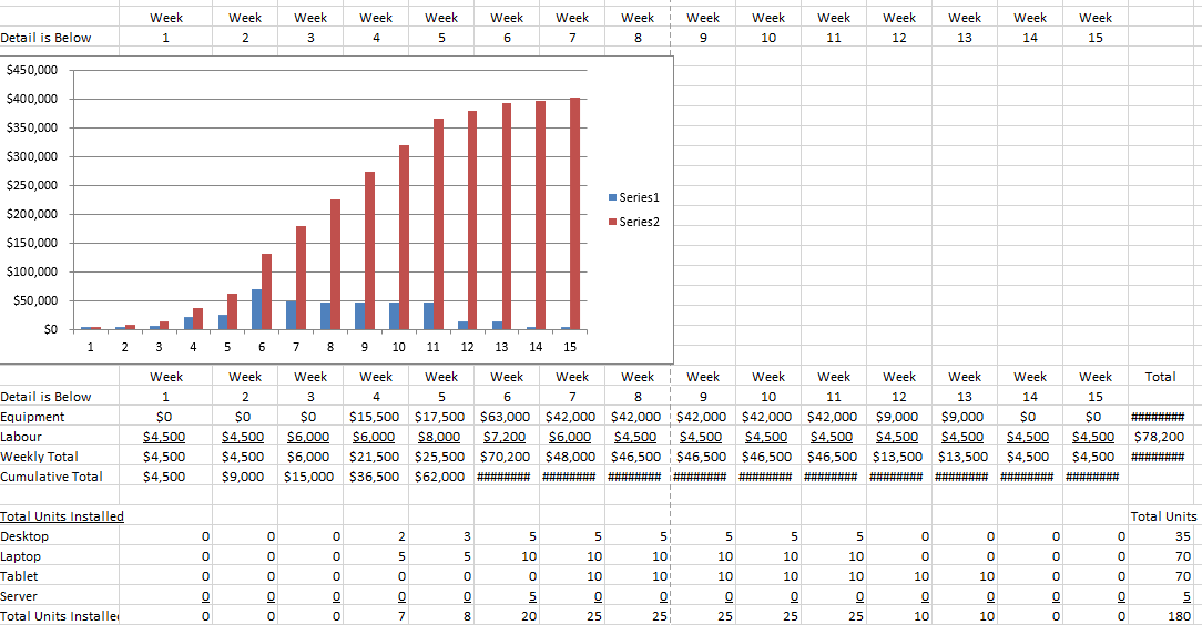
Sheet 1 shows the numeric data entry only. It was started at row 30 to leave space for a data-driven graphic table to be added later.
Sheet 1 15-week budget before a graphic table with input cells yellow. This is the same as sheet one except for the user input cells for unit installations, unit prices, labour days, and labour rates have been shown on a yellow background to ease of use. The other cells are formula-driven.
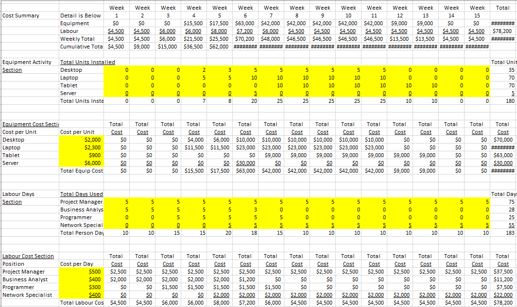
Download Sheet 1 with Yellow Input Cells
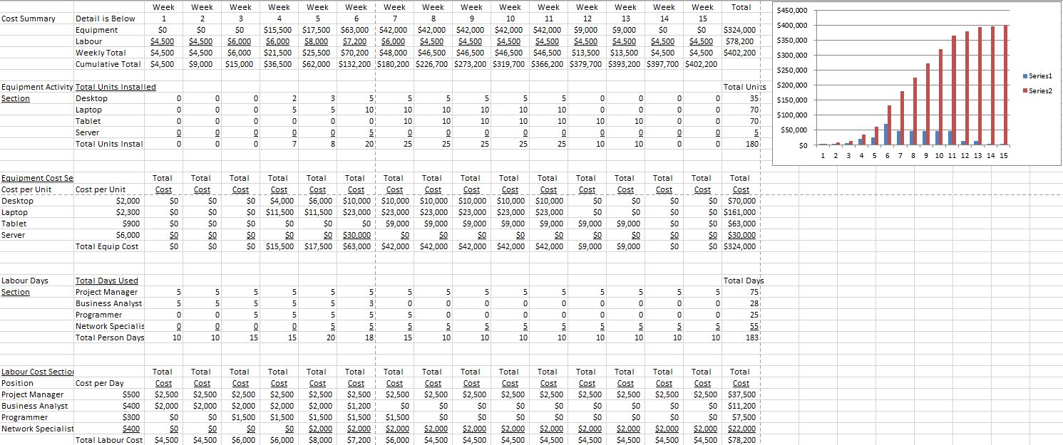
Sheet 2 shows the addition of a data-driven graphic table inserted above the numeric spreadsheet. The instructions for creating the table are:
- Select (curser click on) rows 35 and 36 to include all cells from C35 to Q36
- Click on the Insert tab from the top of the spreadsheet
- Click on the Column Icon
- Select (Click on) the top left 2-D column icon
Advertisement
[widget id=”custom_html-68″]
A two-column graphic showing the weekly planned cost and total cumulative will be superimposed on your spreadsheet. It will not likely be properly positioned or sized to line up with your numeric entries and weekly columns. You will need to use your cursor to grab the corners of the graphic table to stretch and position the table to line up with your numeric entries.
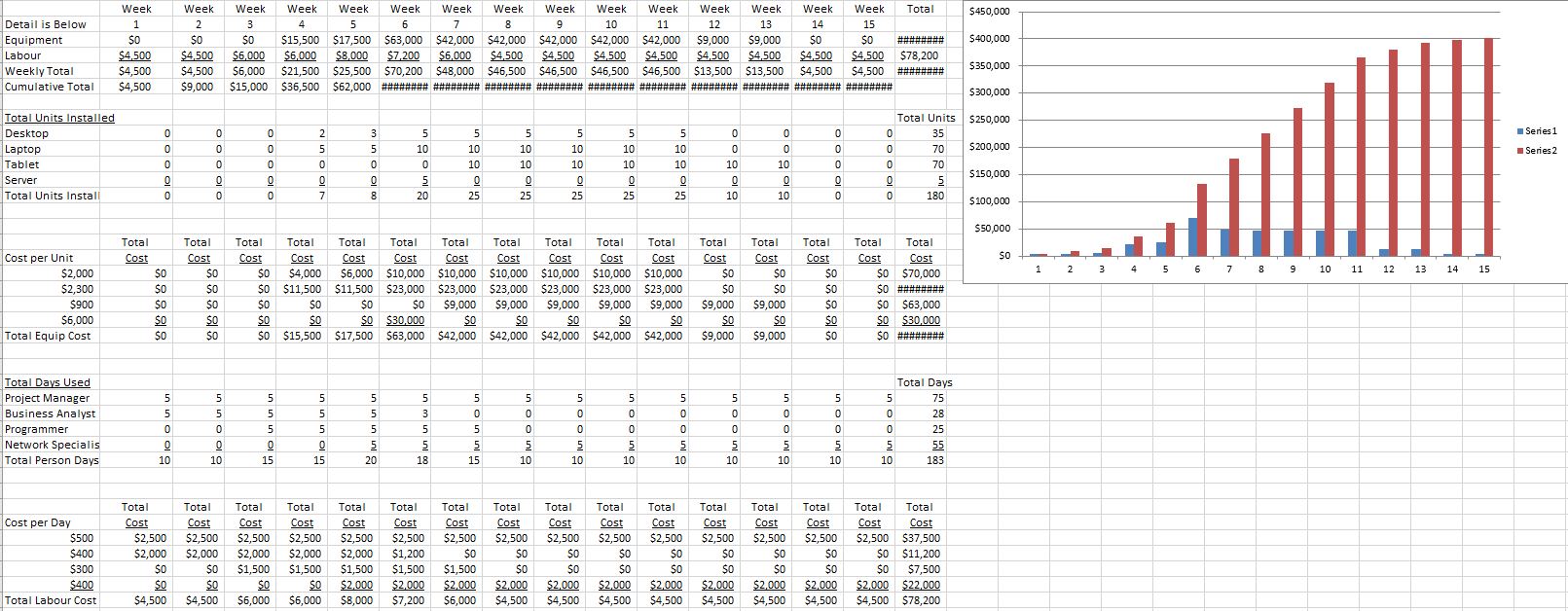
Sheet 3 is the same as spreadsheet 2 after the graphic column table has been stretched and positioned to fit above the numerical data it represents.
Sheet 4 adds a Gantt chart showing key milestones and dates.